Oh hey! Welcome to the community.
Okay, friends. Let’s be honest here. We all like to think we know how to use Excel but if it’s anything more complex than a sum or sort function, we’re not proficient. If you’re looking for Hacks and useful formulas, keep reading! You’ve come to the right place. Both hacks and formulas will be covered in this blog post.
Hacks
AutoSum
Add up a column of numbers quickly by selecting the cells and hitting:
- PC: Alt, =
- Mac: Command, Shift, T
Add a border to a cell or group of cells
Selecting the cells and push:
- PC: Ctrl, Shift, &
- Mac: Command Option 0
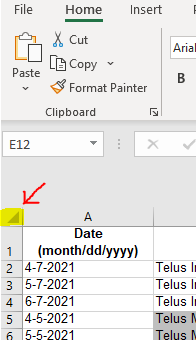
Select all cells
You can select all cells without scrolling. This tip is a huge time saver!
- Just click on the light grey triangle at the top of the table. It’s that easy!
Size a Column
This tip allows you to make the column the largest necessary width without having to figure it out. Move your cursor over the column headings, until you’re between the end of the cell you want to extend and the next cell. The cursor will change to look like this:

Double click on that and the cell will expand to the necessary width.
Cell formatting shortcuts
- Add a $: Ctrl – Shift – 4
- Add a %: Ctrl – Shift – 5
Transferring Information
This tip is a great one when it comes to reports! Transfer cells from your excel document to word and have them automatically update when you make changes! Here are the steps:
- Select the cells in your excel spreadsheet that you want to include in your word document
- Click copy
- In word, find the “Paste Special” option. It’s often under the paste button (top right corner) when you click on the arrow/chevon.
- A pop-up box will come up. Choose Paste Link from the radio buttons and “Microsoft Excel Worksheet Object” from the list.
- Voila! To update the cells in your Word document, right click on the table and choose “Update Link.”
Schedule a demo of eRezLife Software
Formulas
Searching for Specific Values
VLOOKUP – You’ve probably heard of it but have no idea how it works. Let’s try to break it down. VLOOKUP matches the values from the first column to another column. You specify the range and excel will do the rest.
VLOOKUP is easily the recommended formula by those that understand excel to those who do know have a great understanding. As I’m on that lack of understanding side, I’ll refer you to the experts for VLOOKUP instructions. Simon Sez IT does a great job of laying out the process in a simple way.
Sum, Count, Average
These formulas are frequently used when pulling reports in eRezLife. It makes it easy to get numbers for reports or updates without much effort.
- SUM: Allows you to add all of the numbers in a row or column together. =SUM(A1:A8)
- COUNT: Allows you to count the number of cells within a range.=COUNT(A1:A20)
- COUNTIF: Allows you to count the number of times a value is reported within a range (=COUNTIF(A2:A5,”apples”) Apples would be the value in this example and you would sub in your value within the quotes. Click for more COUNTIF examples.
- AVERAGE: Allows you to find the mean average for your range of cells. =AVERAGE(A1:A8)
IF Statements
These are incredible and make a huge difference in your ability to analyze your data. The IF function allows you to easily decipher if the text is valid or false.
For example: =IF(A1>A2, “Meets expectations”, “Not meeting expectations”)
If A1 is greater than A2, excel will add a cell that says Meets expectations. If A2 is greater than A1, excel will report “Not meeting expectations”’
Concatenate
I like this one, partially because my name is in the formula but also because it’s super useful. I even have this one on a post-it note next to my monitor. This formula lets you combine data into one cell without merging the cells. =CONCATENATE(A1 , ” ” , B2) Make sure you don’t forget the “ “, as it creates the space between the data points. You can add as many as you want! =CONCATENATE(A1 , ” ” , B2, “ “, C2, “ “, D2)
Proper
This one is for all the friends in the group that get annoyed by improper formatting. =PROPER(A1:A4), for example, will correct any oddly formatted text within that range.
And
AND was a surprising formula to me and I love it. It will check if certain things are true or false. For example, =AND(C1=”HOMESICK”, B2>3) would output TRUE if C1 is HOMESICK and the value of B2 is greater than 3. You can have it check more values than two as well, simply add them on with another comma.
Let us know what you think!
So that’s it for today! Have a formula that you believe should be highlighted that we missed? Let us know! If you’d like to know more about eRezLife and the exceptional data that is produced using our software, schedule a demo today.
Welcome to the community. We’re glad you’re here.
Sources:
https://www.goskills.com/Excel/Resources/Excel-hacks
https://support.microsoft.com/en-us/office/countif-function-e0de10c6-f885-4e71-abb4-1f464816df34
https://interestingengineering.com/top-10-most-useful-excel-formulas

